Flight Results – Analysis and Presentation

In that chapter you’ll find visualizations in the form of charts based on data collected during the flight. For clarity, time is expressed in seconds. It’s also worth highlighting two key moments: the balloon envelope burst at time t ~ 4300s and the landing at ~ 6250s.

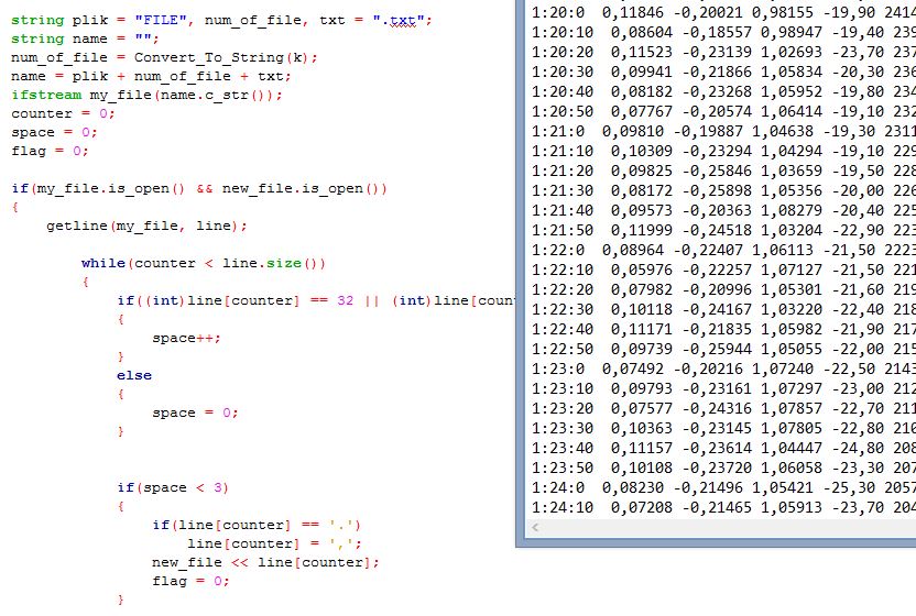
As mentioned in the first article, data was stored on an SD card in buffered form and written as a single string after each cycle of measurements. To process it, I created a simple C++ program that extracted and sorted each variable, saving them into separate files. This allowed me to generate datasets for individual parameters such as temperature or pressure – and create the charts below.

Temperature Inside and Outside the Payload

The external temperature changed very dynamically during the flight. First, around t = 2250s, we can observe an unusual increase in temperature. This is related to UV radiation absorption by ozone molecules, a phenomenon discussed in the first part of the project. This effect persists until the balloon bursts at around 20 km altitude and aligns well with expectations.

Second, there is a sudden temperature drop at the moment of balloon rupture and descent. This can be explained by the high velocity reached by the payload, which likely caused the perceived temperature to be lower than the actual ambient temperature.

The internal temperature behaved more steadily. The payload interior resisted temperature changes for quite some time. Interestingly, the lowest temperature did not occur at peak altitude but several minutes after descent began.

This reveals a key drawback of insulation: while it effectively retains heat during ascent, it also slows down warming when the external temperature becomes higher than inside – for example during descent or after landing. This can lead to moisture formation and potential risks such as short circuits, although I personally haven’t experienced or heard of such cases during such flights.

Pressure

Pressure was another environmental parameter measured during the flight. Due to intentional payload leakiness, internal and external pressure can be considered equal. The leakiness was deliberate to allow pressure equalization. Why? Some of you have probably seen videos of overinflated tires bursting. While the effect here wouldn’t be as spectacular, I preferred to leave a few “air channels” in the payload walls because I wasn’t sure whether a fully sealed payload might rupture, or whether the pores in the polystyrene structure would be sufficient for pressure equalization. To this day, I still don’t know – and I continue to keep the payload slightly unsealed 🙂

It’s worth noting an interesting detail. The lowest recorded pressure during the flight was about 6000 Pa (60 hPa), measured at peak altitude – which matches expectations. However, the sensor manufacturer specifies a minimum operating pressure of 200 hPa. That’s a difference of 140 hPa, which initially raised concerns about measurement accuracy below the specified range. Fortunately, comparison with data from other teams (some using different sensors) confirmed that the readings were correct. This suggests that the module is capable of measuring even such extreme pressure values.

Humidity

Humidity can significantly affect electronic systems, which is why it was also measured during the mission. The chart shows humidity changes over time.

Two key moments can be observed. Around t = 300 s, there is a rapid increase in humidity – later confirmed by onboard footage, as the balloon was passing through lower cloud layers. After some time, humidity drops almost to zero and remains at that level even shortly after the balloon bursts.

The second important event is a sharp increase in humidity during descent. This was likely caused by the payload interior warming up much more slowly than the surrounding air. As the payload descended into warmer and more humid atmospheric layers, its internal components remained cold. Under such conditions, surface temperatures could drop below the dew point, leading to condensation.

After opening the enclosure, small water droplets were still visible on the PCB. Despite this, the electronics continued to function correctly until my arrival to pick the payload up.

G-forces during flight

At first glance, it’s clear that the payload flight was not stable. The data shows that the payload experienced significant movement and rotation, which is also confirmed by flight camera.

These uncontrolled rotations directly impact the quality of captured photos and videos. This makes an opportunity for improvement – for example, by implementing stabilization systems such as reaction wheels or weighted arms to reduce rotational motion.

However, such solutions increase payload mass, which in turn requires more lifting gas (e.g., helium). The additional buoyant force must compensate for the increased weight, as the difference between these forces determines the ascent rate.

It’s also possible to clearly identify the moment of balloon burst – when the resultant force drops significantly below 1g. This is caused by rapid deceleration of the payload. After this moment, force components fluctuate dynamically until landing, after which they stabilize.

Altitude

Altitude was not measured directly but calculated based on pressure readings using a formula provided by the sensor manufacturer.

The calculated altitude more or less matches GPS data. At peak altitude, the difference between pressure-based and GPS measurements is less than 1 km. This indicates that such calculations can serve as a useful indicator – but only within the pressure sensor’s reliable operating range. At higher altitudes, GPS is likely the better solution.

Some irregularities can be observed around t = 250 s, t = 2400 s, and t = 3600 s. These deviations are caused by inaccuracies in pressure measurements at those moments.

Ascent and Descent Rate

Another calculated parameter is the ascent and descent rate. While not as precise as GPS measurements, the results are reliable enough for analysis – which is also supported by data from other stratospheric missions.Velocity was calculated based on the basic physical definition – distance traveled over time.

Based on experience from similar missions, applying these formulas with a small Δt (in this case 10 seconds – the data logging interval) is justified. Δs represents the change in altitude calculated from pressure differences over that time interval.

During ascent, a decreasing trend in velocity is visible. This is due to decreasing pressure and thus decreasing buoyant force. Since gravitational force remains constant, the net upward force decreases with altitude.

At the moment of balloon burst, a rapid increase in velocity can be observed, along with a change in direction (negative values). Based on the data, the impact speed upon landing can be estimated at around 25 km/h.

Additionally, the data shows the effect of air resistance on descent rate – especially after the balloon reaches low altitudes.

Light Intensity

An experiment aimed at measuring the relationship between sunlight intensity and altitude. Unfortunately, this experiment failed. The data is essentially noise, as shown in the chart. This was caused by an incorrect data processing method.

Measurements were taken continuously, and the average value was calculated before saving to the SD card. This led to two major issues.

First, too many samples may have been taken when the sensor was not facing the Sun, significantly lowering the average value. Tests showed that even a slight deviation from the direction of sunlight causes large measurement differences.

Second, averaging itself turned out to be a poor approach. A better solution would be to record maximum values or use the median over a defined sample set within a given time interval.

Due to these factors, the experiment must be considered unsuccessful. However, even failures provide valuable insights that can help improve data collection algorithms and produce more accurate results in the future.

Project Summary

This was my first project of this scale. I worked on it alone because, as mentioned in previous posts, I wanted to combine my passion, fulfill a dream of collecting data and images from high altitude, and – most importantly – use the project as my engineering thesis to graduate.

The project was demanding at every stage and required a lot of effort, but I’m satisfied with what I achieved. No one said it would be easy, but experiences like this make you grow.

Even though I now see many ways it could have been done better, the fact that I completed it means I now know what I would improve next time 😊

That’s why I believe it’s worth taking risks and starting something – even if it doesn’t work out perfectly the first time. It will almost certainly be better the next time, because nothing teaches like practice. Of course… supported by theory 😄

Thanks for reading all the way to the end. See you next time!